9. Running a Machine Learning Analysis

Here, we will run a quick machine learning analysis on this age dataset. Particularly, we're going to focus on two applications, clustering and age prediction. As examples, we're going to show that similar ages cluster together, and demonstrate that we can make a model that predicts someone's age.

First, if you want this analysis to run faster, but have lower accuracy, prune some of the CpGs, in this case I'm saving 25000 of them while retaining only 35% of the samples:

>>> from pymethylprocess.MethylationDataTypes import MethylationArray
>>> sample_p = 0.35
>>> methyl_array=MethylationArray.from_pickle("train_methyl_array.pkl")
>>> methyl_array.subsample("Age",frac=None,n_samples=int(methyl_array.pheno.shape[0]*sample_p)).write_pickle("train_methyl_array_subsampled.pkl")
>>> methyl_array=MethylationArray.from_pickle("val_methyl_array.pkl")
>>> methyl_array.subsample("Age",frac=None,n_samples=int(methyl_array.pheno.shape[0]*sample_p)).write_pickle("val_methyl_array_subsampled.pkl")
>>> methyl_array=MethylationArray.from_pickle("test_methyl_array.pkl")
>>> methyl_array.subsample("Age",frac=None,n_samples=int(methyl_array.pheno.shape[0]*sample_p)).write_pickle("test_methyl_array_subsampled.pkl")
>>> pymethyl-utils feature_select_train_val_test -n 25000

The previous step is not necessary but is a neat trick, enacted via the .subsample() method of MethylationArray.

Then, we'd want to UMAP transform the data using (make sure to load the saved MethylationArrays again as train_methyl_array, val_methyl_array, and test_methyl_array respectively):

from umap import UMAP
umap = UMAP(n_components=100)
umap.fit(train_methyl_array.beta)
train_methyl_array.beta = pd.DataFrame(umap.transform(train_methyl_array.beta.values),index=train_methyl_array.return_idx())
val_methyl_array.beta = pd.DataFrame(umap.transform(val_methyl_array.beta),index=val_methyl_array.return_idx())
test_methyl_array.beta = pd.DataFrame(umap.transform(test_methyl_array.beta),index=test_methyl_array.return_idx())

We just replaced the CpGs of the beta values with 100 UMAP components, the dimensionality reduction model trained on the training data.

UMAP works well with HDBScan in conjunction https://umap-learn.readthedocs.io/en/latest/clustering.html, so let's cluster using HDBScan if it is installed, if not you can get it here: https://hdbscan.readthedocs.io/en/latest/how_hdbscan_works.html. We'll just run this on our training data:

from sklearn.decomposition import PCA
import matplotlib, matplotlib.pyplot as plt
import seaborn as sns
from seaborn import cubehelix_palette
sns.set()
def reduce_plot(data, labels, legend_title):
    np.random.seed(42)
    plt.figure(figsize=(8,8))
    t_data=pd.DataFrame(PCA(n_components=2).fit_transform(data),columns=['z1','z2'])
    t_data[legend_title]=labels
    sns.scatterplot('z1','z2',hue=legend_title, cmap=cubehelix_palette(as_cmap=True),data=t_data)

model = HDBSCAN(algorithm='best')
train_predicted_clusters = model.fit_predict(train_methyl_array.beta.astype(np.float64))
reduce_plot(train_methyl_array.beta, train_methyl_array.pheno['Age'].values,'Age')
reduce_plot(train_methyl_array.beta, train_predicted_clusters,'Cluster')

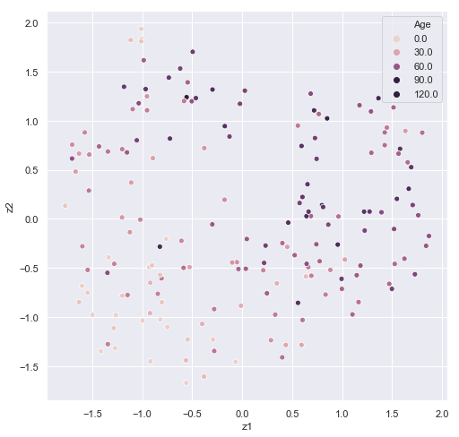
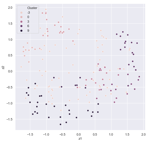
It's easy to see some correspondence between age and cluster. In HDBSCAN, we would want to filter out the data with the -1 cluster labels in future predictions. Some sets of ages appear to correspond to a particular cluster.

train_methyl_array.pheno['Cluster']=train_predicted_clusters
output_data=train_methyl_array.pheno.groupby('Cluster')['Age'].agg([np.mean,len])

Cluster	mean	n
-1	50.8971	68
0	43.5	10
1	55.3529	17
2	56	8
3	72.4286	7
4	55.375	8
5	58.75	8
6	59.2353	17
7	36.3333	6
8	25.4074	27

After an unsupervised analysis, we may want to try something more supervised and actually predict age in the other two sets. This can be accomplished either by setting up your own pipeline with the convenient data setup, or by calling the general_machine_learning part of the package. Officially, functionality can be accessed on the command line using the pymethyl-basic-ml command and (-h) for help in running. I'll illustrate how to run the module but leave it as a task for the user to run:

from sklearn.ensemble import RandomForestRegressor
from sklearn.metrics import r2_score

y_pred = {}
scores={}
model=MachineLearning(RandomForestRegressor,options={})
model.fit(train_methyl_array,val_methyl_array,'Age')
y_pred['train']=model.predict(train_methyl_array)
y_pred['val']=model.predict(val_methyl_array)
y_pred['test']=model.predict(test_methyl_array)

scores['train']=r2_score(train_methyl_array.pheno['Age'],y_pred['train'])
scores['val']=r2_score(val_methyl_array.pheno['Age'],y_pred['val'])
scores['test']=r2_score(test_methyl_array.pheno['Age'],y_pred['test'])
scores

A reminder that this is a severely limited dataset, and limiting to only 100 UMAP components. With the right data and right model, even utilizing all of the CpGs, predictive accuracy should skyrocket. One could also concatenate the validation data to the training data and train using cross validation. The machine learning module adds the convenience of being able to input a MethylationArray object and run hyperparameter scans. Feature requests are welcome.

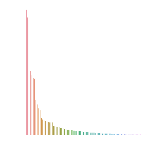
We can also get Gini Indexes that label how important each UMAP embedding was to the prediction. If we did away with the UMAP embedding layer and ran the model in the same manner, we'd get this value for each CpG.

data=pd.DataFrame(model.model.feature_importances_,columns=['Importance'])
data=data.sort_values('Importance').iloc[::-1]
data['sample']=np.arange(len(data.index))

plt.figure(figsize=(5,5))
sns.barplot('sample','Importance',data=data)
plt.axis('off')

Here's what I found when running the model (again, tuning hyperparameters via some grid search or hyperparameter optimization method may be essential, maximizing validation set's score):