pygridmappr

A faithful Python implementation of the R package gridmappr by Roger Beecham.

Table of Contents

• Overview
• Features
• Installation
• Quick Start
• Core Function
• Mathematical Approach
• Examples
• Demonstration Gallery
• Design Philosophy
• Differences from R Implementation
• References
• License
• Citation
• Contributing
• Acknowledgments

Overview

pygridmappr automates the generation of small multiple gridmap layouts. Given a set of geographic point locations, it creates a grid with specified row and column dimensions, placing each point in a grid cell such that the distance between points in geographic space and grid space is minimized.

This implementation maintains full feature parity with the original R package and replicates the mathematical logic as faithfully as possible.

Features

• ✅ Algorithm replication: Uses Hungarian algorithm (linear sum assignment) for optimal point-to-grid allocation
• ✅ Compactness parameter: Control trade-off between geographic fidelity and grid compactness (0-1 scale)
• ✅ Spacer cells: Constrain allocation by excluding specific grid cells
• ✅ Quality metrics: Compute RMSE, mean distance, and other quality measures
• ✅ Visualization tools: Compare geographic and grid layouts side-by-side
• ✅ Deterministic results: Reproducible allocations for identical inputs

Installation

# From source (recommended for development)
git clone https://github.com/TMFNK/pygridmappr
cd pygridmappr
pip install -e .

# Or via pip (when available)
pip install pygridmappr

Requirements

• Python ≥ 3.7
• Core Dependencies:
  • numpy ≥ 1.19.0
  • pandas ≥ 1.1.0
  • scipy ≥ 1.5.0
  • matplotlib ≥ 3.3.0

Development Installation

For contributors and developers:

git clone https://github.com/TMFNK/pygridmappr
cd pygridmappr
pip install -e ".[dev]"

Quick Start

import pandas as pd
from pygridmappr import points_to_grid, visualize_allocation

# Create point data
pts = pd.DataFrame({
    'area_name': ['A', 'B', 'C', 'D'],
    'x': [0, 100, 100, 0],
    'y': [0, 0, 100, 100]
})

# Allocate to 2×2 grid
result = points_to_grid(pts, n_row=2, n_col=2, compactness=0.5)

# Visualize
fig, axes = visualize_allocation(result, n_row=2, n_col=2)

Core Function: points_to_grid()

points_to_grid(
    pts: pd.DataFrame,
    n_row: int,
    n_col: int,
    compactness: float = 1.0,
    spacers: Optional[List[Tuple[int, int]]] = None
) -> pd.DataFrame

Parameters

• pts: DataFrame with columns 'x' and 'y' (required), optionally 'area_name' or other identifiers
• n_row: Number of grid rows (must be ≥ 1)
• n_col: Number of grid columns (must be ≥ 1)
• compactness: Value between 0 and 1:
  • 0.5: Preserves scaled geographic layout
  • 1.0: Allocates toward grid center (compact cluster)
  • 0.0: Allocates toward grid edges
• spacers: List of (row, col) tuples using 1-based indexing with origin (1,1) at bottom-left (matches R convention)

Returns

DataFrame with added columns:

• row: Grid row assignment (1-based)
• col: Grid column assignment (1-based)
• grid_x: X coordinate of grid cell center
• grid_y: Y coordinate of grid cell center

Mathematical Approach

The algorithm minimizes the total squared distance between:

1. Geographic positions (scaled to grid bounds)
2. Grid cell positions

Cost Matrix

For each point i and grid cell j:

C[i,j] = (x_scaled[i] - x_grid[j])² + (y_scaled[i] - y_grid[j])²

Compactness Adjustment

When compactness ≠ 0.5, costs are modified based on distance from grid center:

penalty = -2(compactness - 0.5) × normalized_distance_from_center[j]
C[i,j] += penalty × mean(C[i,:])

• compactness > 0.5: Reduces cost for cells near center (attraction)
• compactness < 0.5: Increases cost for cells near center (repulsion)

Assignment

The optimal assignment is found using scipy.optimize.linear_sum_assignment (Hungarian algorithm), which solves:

minimize Σᵢ C[i, assignment[i]]

subject to:

• Each point assigned to exactly one cell
• Each cell contains at most one point

Examples

Example 1: Basic Allocation

from pygridmappr import points_to_grid, generate_sample_points

# Generate random points
pts = generate_sample_points(n_points=20, pattern='random', seed=42)

# Allocate with geographic preservation
result = points_to_grid(pts, n_row=5, n_col=5, compactness=0.5)

Example 2: Compactness Comparison

from pygridmappr import compare_compactness

fig, axes = compare_compactness(
    pts,
    n_row=6, n_col=6,
    compactness_values=[0.0, 0.5, 1.0]
)

Example 3: Using Spacers

# Define spacers to create separation (e.g., island from mainland)
spacers = [
    (1, 11), (2, 11), (3, 11),  # Bottom-right corner
    (1, 10), (2, 10)
]

result = points_to_grid(
    pts,
    n_row=13, n_col=12,
    compactness=0.6,
    spacers=spacers
)

Example 4: Quality Metrics

from pygridmappr import compute_allocation_quality

quality = compute_allocation_quality(result)
print(f"RMSE: {quality['rmse']:.3f}")
print(f"Mean distance: {quality['mean_distance']:.3f}")
print(f"Max distance: {quality['max_distance']:.3f}")

Demonstration Gallery

The package includes comprehensive demonstrations that showcase the key features and capabilities of the gridmappr algorithm. These examples illustrate the mathematical principles and practical applications of the grid allocation method.

Quick Start

Run the complete demonstration suite:

cd examples
python demo.py

This generates five professional visualizations that demonstrate different aspects of the algorithm:

---

Demo 1: Basic Point Allocation

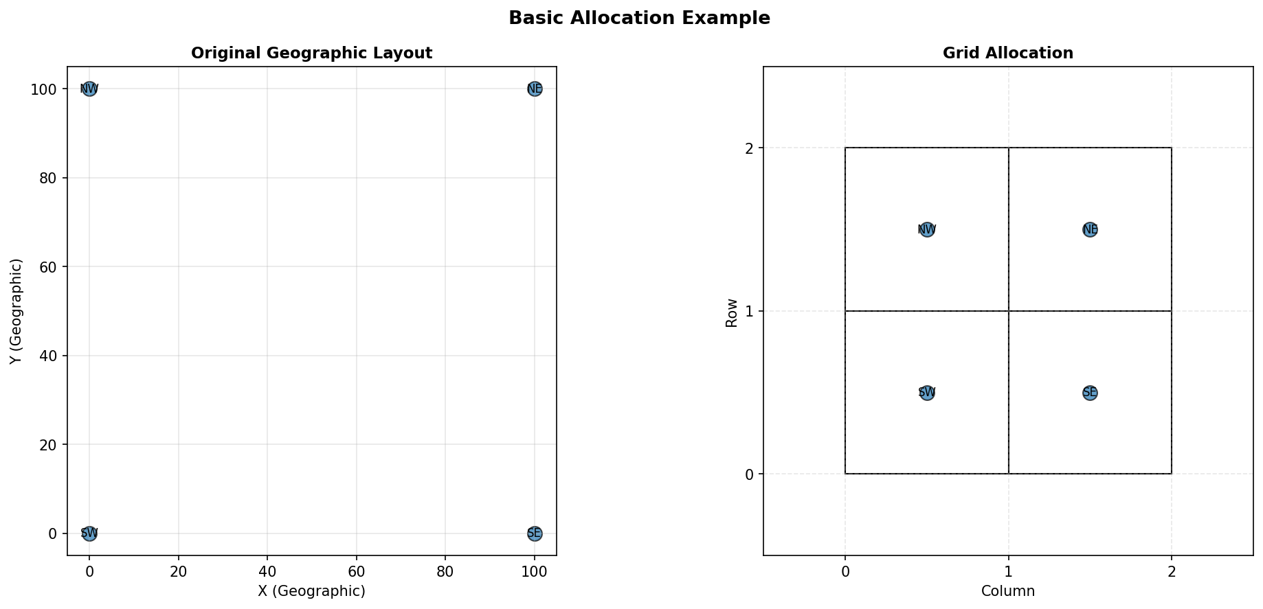
Figure 1: Basic 2×2 grid allocation demonstrating optimal assignment of four corner points to grid cells while preserving geographic relationships. The algorithm minimizes total squared distance between original geographic positions and grid cell centers.

---

Demo 2: Compactness Parameter Effect

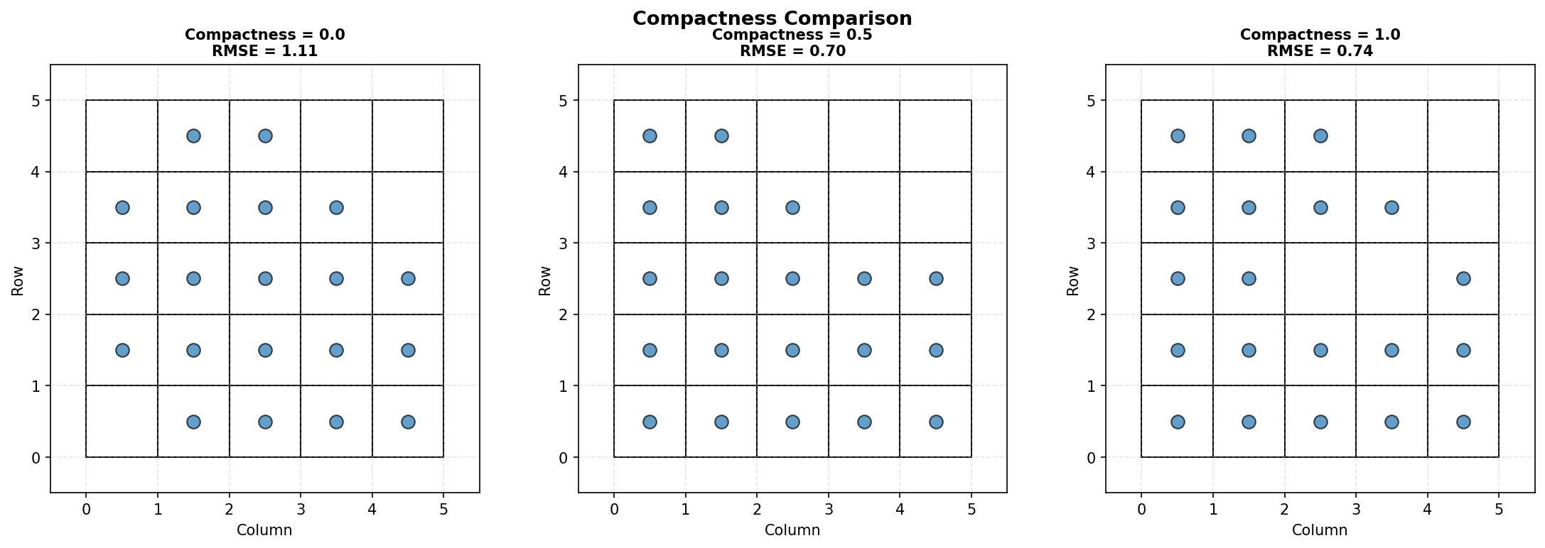
Figure 2: Systematic comparison of compactness parameter effects (0.0, 0.5, 1.0). The compactness parameter controls the trade-off between geographic fidelity and grid clustering: lower values preserve spatial relationships while higher values create more compact, centralized clusters.

---

Demo 3: Spacer Constraints

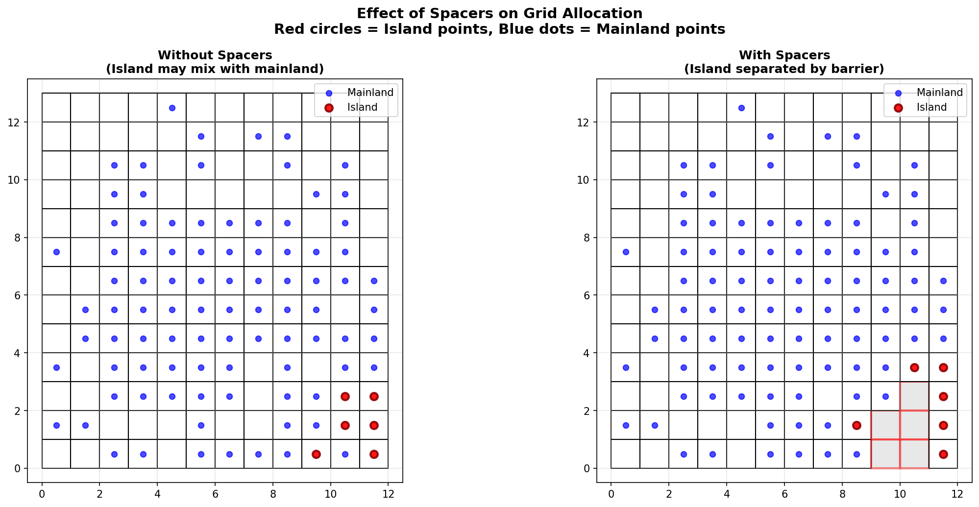
Figure 3: Demonstration of spacer constraints for geographic separation. Left panel shows unconstrained allocation allowing mainland-island mixing; right panel shows allocation with spacer barriers creating forced separation, effectively mimicking the geographic isolation of Corsica from mainland France.

---

Demo 4: Geographic Pattern Analysis

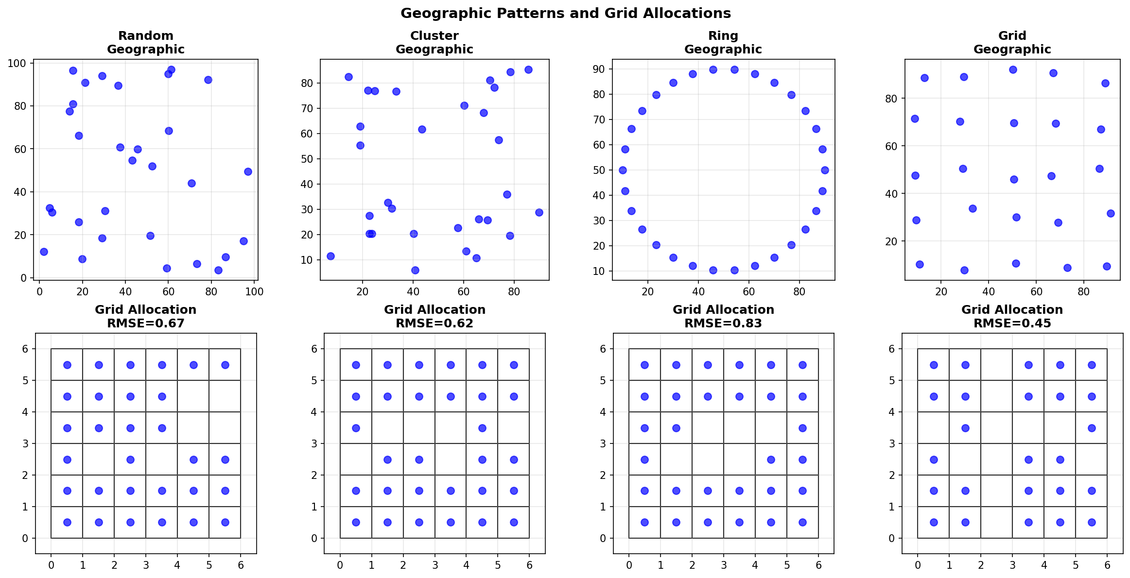
Figure 4: Comparative analysis of different geographic input patterns (random, cluster, ring, grid) and their transformation into grid layouts. Each column shows the original geographic distribution (top row) and resulting grid allocation (bottom row) with quantitative RMSE quality metrics.

---

Demo 5: Grid Size Optimization

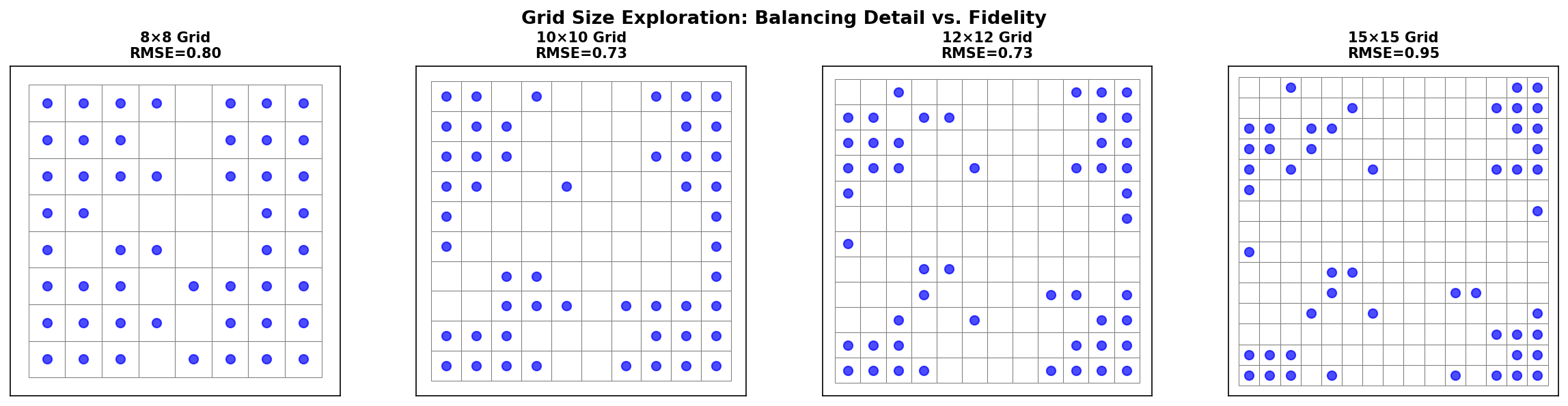
Figure 5: Systematic exploration of grid size effects on allocation quality. Analysis shows how different grid dimensions (8×8, 10×10, 12×12, 15×15) balance between available graphic space and geographic fidelity, with quantitative RMSE measurements for each configuration.

Design Philosophy

This implementation prioritizes accuracy over optimization. The code structure and logic closely mirror the original R implementation to ensure:

1. Mathematical fidelity: Exact replication of cost calculations and compactness effects
2. Reproducibility: Deterministic results for research and documentation
3. Transparency: Clear documentation of algorithm steps with references

Differences from R Implementation

• Language: Python instead of R
• Solver: scipy.optimize.linear_sum_assignment instead of R's linear programming solver
• Visualization: matplotlib instead of ggplot2
• Data structures: pandas DataFrame instead of tibble

Core algorithm behavior is identical.

References

Original R Package

• Beecham, R. (2021). gridmappr: Gridmap Allocations with Approximate Spatial Arrangements. https://github.com/rogerbeecham/gridmappr

Publications

• Beecham, R., Dykes, J., Hama, L. and Lomax, N. (2021). On the Use of 'Glyphmaps' for Analysing the Scale and Temporal Spread of COVID-19 Reported Cases. ISPRS International Journal of Geo-Information, 10(4), 213. https://doi.org/10.3390/ijgi10040213

• Beecham, R. and Slingsby, A. (2019). Characterising labour market self-containment in London with geographically arranged small multiples. Environment and Planning A: Economy and Space, 51(6), 1217–1224. https://doi.org/10.1177/0308518X19850580

Inspiration

• Wood, J. Observable notebooks on Linear Programming and Gridmap Allocation

License

AGPL-3.0 License (matching original R package)

Citation

If you use this package, please cite the original R package:

@software{beecham2021gridmappr,
  author = {Beecham, Roger},
  title = {gridmappr: Gridmap Allocations with Approximate Spatial Arrangements},
  year = {2021},
  url = {https://github.com/rogerbeecham/gridmappr}
}

Contributing

Contributions are welcome! Please ensure any changes maintain mathematical fidelity with the original R implementation.

Acknowledgments

This Python implementation is based on Roger Beecham's excellent R package gridmappr. All credit for the algorithm design and innovation goes to Roger Beecham and Jo Wood.