5. Examples
ReporTree can facilitate the routine surveillance and outbreak investigation of bacterial pathogens, such as foodborne pathogens. Below, we provide a simple example of the usage of ReporTree to rapidly identify and characterize potential Listeriosis outbreaks. With a single command, ReporTree builds a MST from cgMLST data and automatically extracts genetic clusters at three high resolution levels (<=4, <=7, <=14 allelic differences), and provides comprehensive reports about the sample collection (e.g., ST sequence count/frequency per year, etc). In this command line, we also provide a table with clustering information at 1, 4 and 7 allele distances of a previous ReporTree run in order to maintain cluster names.
Example using a cgMLST allelic matrix (built using Moura’s cgMLST schema and chewBBACA allele calling) and artificially generated metadata.
NOTE: All input and output data used/generated in this example are available at examples/Listeria/.
python reportree.py -m input/Listeria_metadata.tsv -a input/Listeria_alleles.tsv --loci-called 0.95 --columns_summary_report country,n_country,source -out output/Lm --analysis grapetree --partitions2report 4,7,15 --nomenclature-code 150,7,4,country --nomenclature-file input/Listeria_nomenclature.tsv --sample_of_interest sample_0269,sample_0675,sample_0010In the partitions_summary.tsv table, ReporTree lists the identified clusters of highly closely related strains (e.g. clusters at <=4 or <=7 allelic differences) that may represent potential outbreaks, and their full characterization according to any user-defined metadata variable (e.g. country distribution, source type, timespan, etc.). Moreover, as a a previous nomenclature was provided for the clusters obtained at 4 and 7 allele distances, this table also comprises information about the nomenclature change.

Users can further interactively visualize and explore the ReporTree derived clusters by uploading the metadata table with additional columns comprising information on the genetic clusters (metadata_w_partitions.tsv) table together with the allele profile matrix (alleles_4_grapetree.tsv) using a local version of GrapeTree (the dataset is visualized client-side in the browser).

Large-scale genetic clustering and linkage to antibiotic resistance data (e.g. Neisseria gonorrhoeae)
To show how ReporTree can enhance genomics surveillance and quickly identify/characterize genetic clusters, here, we reproduce part of the extensive genomics analysis of the bacterial pathogen Neisseria gonorrhoeae performed by Pinto et al., 2021 using a single command line. In this study, 3,791 N. gonorrhoeae genomes from isolates collected across Europe were analyzed with a cgMLST approach. The input allele matrix can be found in Zenodo and the associated metadata in the supplementary material 1.
NOTE: All output data generated in this example are available at examples/Neisseria/.
python reportree.py reportree.py -m input/NG_Metadata_NEW.tsv -a input/Allelic_profile_matrix_MScgMLST_822_loci_3791_isolates_NEW.tab --output output/NG_822 --method MSTree --n_proc 1 --matrix-4-grapetree --columns_summary_report n_sequence,first_seq_date,last_seq_date,timespan_days,country,n_country,MLST --partitions2report stability_regions -AdjW 0.99 -n 9 --metadata2report country --analysis grapetree --nomenclature-file input/NG_nomenclature.tsv --nomenclature-code 39This command line outputs:
- List of regions of cluster stability
#Stability regions of the Adjusted Wallace coefficient for  NG_822_metrics.tsv
#using a threshold of  0.99  and minimum number of required observations of  9
#block_id	first_partition	last_partition	len_block
block_8	MST-40x1.0->MST-39x1.0	MST-54x1.0->MST-53x1.0	15
block_14	MST-79x1.0->MST-78x1.0	MST-193x1.0->MST-192x1.0	115
block_17	MST-207x1.0->MST-206x1.0	MST-221x1.0->MST-220x1.0	15
block_19	MST-232x1.0->MST-231x1.0	MST-243x1.0->MST-242x1.0	12
block_20	MST-245x1.0->MST-244x1.0	MST-254x1.0->MST-253x1.0	10
block_21	MST-256x1.0->MST-255x1.0	MST-279x1.0->MST-278x1.0	24
block_23	MST-286x1.0->MST-285x1.0	MST-294x1.0->MST-293x1.0	9
block_26	MST-300x1.0->MST-299x1.0	MST-317x1.0->MST-316x1.0	18
block_29	MST-333x1.0->MST-332x1.0	MST-355x1.0->MST-354x1.0	23
block_31	MST-363x1.0->MST-362x1.0	MST-371x1.0->MST-370x1.0	9
block_34	MST-383x1.0->MST-382x1.0	MST-399x1.0->MST-398x1.0	17
block_35	MST-401x1.0->MST-400x1.0	MST-413x1.0->MST-412x1.0	13
block_36	MST-415x1.0->MST-414x1.0	MST-425x1.0->MST-424x1.0	11
block_41 MST-453x1.0->MST-452x1.0 MST-471x1.0->MST-470x1.0 19- Updated metadata table with clustering information for the first partition of each stability region
TIP: this table can be used for visualization with GrapeTree (corresponding to Figures 1a and 1b of Pinto et al., 2021)
- Summary report for the genetic clusters of the higher level of stability (Table 1 of Pinto et al., 2021)

- Summary report for the genetic clusters of the lower level of stability (Table 2 of Pinto et al., 2021)

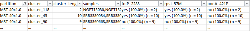
To include in these summary reports the distribution and occurrence of the genetic determinants involved in antimicrobial resistance, as shown in Figure 3 of Pinto et al., 2021, the command line described above just needed to comprise the name of the columns with this information in the '--columns_summary_report' argument.
python reportree.py reportree.py -m input/NG_Metadata_NEW.tsv -a input/Allelic_profile_matrix_MScgMLST_822_loci_3791_isolates_NEW.tab --output output/NG_822 --method MSTree --n_proc 1 --matrix-4-grapetree --columns_summary_report n_sequence,first_seq_date,last_seq_date,timespan_days,country,n_country,MLST,NG_MAST,NG_STAR,folP_228S,rpsJ_57M,ponA_421P,porB_type,porB_120K,porB_121D,porB_121N,rpoB_553N,pro_mtrR_35Adel,pro_mtrR_A38C,mtrR_45D,mtrR_A39T,mtrR_R44H,gyrA_91F,gyrA_95G,gyrA_95N,parC_86N,parC_87I,parC_87R,parC_88P,parC_91K,penA_311V,penA_312M,penA_316T,penA_483S,penA_501V,penA_542S,penA_545S,penA_551S,23SrRNA_A204G,23SrRNA_C2597T,16SrRNA_C1184T,tetM,blaTEM --partitions2report stability_regions -AdjW 0.99 -n 9 --metadata2report country --analysis grapetree --nomenclature-file input/NG_nomenclature.tsv --nomenclature-code 39
ReporTree is currently applied to generate weekly reports about SARS-CoV-2 variant circulation in Portugal (https://insaflu.insa.pt/covid19/). Below, we give some examples on how to rapidly generate key surveillance metrics taking as input metadata tables (tsv format) and rooted divergence (SNP) trees (newick format) provided for download in regular Nextstrain (auspice) builds, such as those maintained by the National Institute of Health Dr. Ricardo Jorge, Portugal (INSA) at https://insaflu.insa.pt/covid19/.
Example using the INSA sequence dataset (“Nov2021-current”) collected from November 1st, 2021 to February 8th, 2022 (downloaded on February 22nd, 2022)
NOTE: All input and output data used/generated in this example are available at examples/SARS-CoV-2/.
1) Generation of an overview report with the number of sequences, temporal (first_seq_date,last_seq_date,timespan_days) and geographic (Health Region, division and location) distribution, and national weekly relative frequencies (representative sampling) for each Pango lineage and Nextstrain Clade:
python reportree.py -m nextstrain_ncov_PT_INSA_since_Nov2021_release_2022-02-22.tsv --columns_summary_report n_strain,first_seq_date,last_seq_date,timespan_days,n_Health_region,Health_region,division,n_division,n_location,lineage,clade_membership --metadata2report lineage,clade_membership,Health_region -f 'country == Portugal;Representative_sampling == Weekly' --frequency-matrix 'lineage,iso_week;clade_membership,iso_week' --count-matrix 'lineage,iso_week;clade_membership,iso_week' -out ReporTree_ncov_PT_lineage_clade_overviewNOTE: ‘iso_week’ is automatically inferred from the ‘date’ column
Example of a metadata summary report for Nextstrain clades:
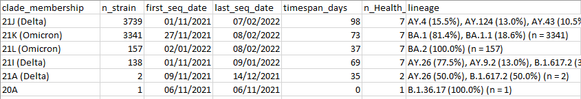
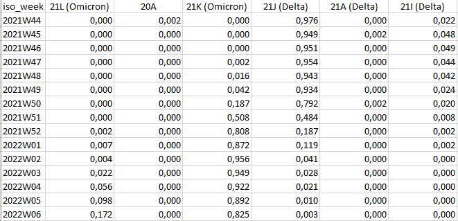
Example of output of the Nextstrain clade frequency per iso_week:
2) Generation of reports on Pango lineage/Nextstrain Clade weekly relative frequencies (and absolute sequence counts) at Regional level (representative sampling) for the last five ISO weeks (2022-W02 to 2022-W06):
NOTE: ‘iso_week’ is automatically inferred from the ‘date’ column
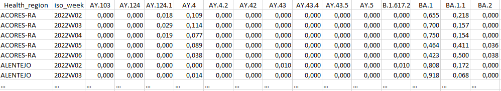
python reportree.py -m nextstrain_ncov_PT_INSA_since_Nov2021_release_2022-02-22.tsv --columns_summary_report n_strain,n_originating_lab --metadata2report Health_region,iso_week -f 'country == Portugal;Representative_sampling == Weekly;iso_week == 2022W02,2022W03,2022W04,2022W05,2022W06' --frequency-matrix 'lineage,Health_region:iso_week;clade_membership,Health_region:iso_week' --count-matrix 'lineage,Health_region:iso_week;clade_membership,Health_region:iso_week;Health_region,iso_week' -out ReporTree_ncov_PT_lineage_clade_reg_freqExample of output of the lineage frequency per iso_week at regional level:
3) Identification of genetic clusters at user-specified clustering methods and SNP thresholds and their characterization according to any epidemiologically/biologically relevant indicators included in metadata (such as timespan, vaccination status, geography or number of S1 mutations):
python reportree.py -m nextstrain_ncov_PT_INSA_since_Nov2021_release_2022-02-22.tsv -t nextstrain_ncov_PT_INSA_since_Nov2021_release_2022-02-22.nwk --columns_summary_report n_strain,lineage,clade_membership,first_seq_date,last_seq_date,timespan_days,n_Health_region,Health_region,S1_mutations --metadata2report S1_mutations --method-threshold root_dist-25-69,avg_clade-1,max_clade-2 -out ReporTree_ncov_PT_get_clustersExample of output of the cluster metadata report:
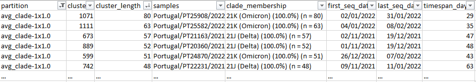
Users can further interactively visualize and explore the ReporTree derived clusters by uploading the original newick tree (e.g. rooted SNP-scaled tree) together with the metadata table with additional columns comprising information on the genetic clusters (metadata_w_partitions.tsv) at auspice.us (the dataset is visualized client-side in the browser).