CloudCal is an open-source Shiny application for building and applying quantitative calibrations for X-ray fluorescence (XRF) spectrometers. It supports multiple instrument manufacturers, file formats, and calibration algorithms ranging from simple linear regression to advanced machine learning models.
- Features
- Supported Instruments
- Supported File Formats
- Calibration Models
- Installation
- Quick Start
- Data Format Requirements
- The .quant File Format
- How It Works
- Citation
- References
- Interactive spectrum visualization with zoom and pan
- Automatic and manual energy calibration
- Spectral deconvolution using iterative least squares
- Multiple compression levels (100 eV, 50 eV, 25 eV bins)
- Log, exponential, and velocity transformations
- K-alpha, K-beta, L-alpha, L-beta, and M-line support for 88 elements (Ne through U)
- Multiple peak calculation methods: Gaussian, Split, First, Second
- Custom line definition support
- Covariance matrix visualization
- Time normalization
- Total counts normalization
- Compton scatter normalization (adjustable energy range)
- Region of Interest (ROI) normalization with Raw/Baseline/Net options
- LiveTime normalization for dead time correction
- Cross-validation methods: k-fold, Bootstrap, 0.632 Bootstrap, Leave-One-Out (LOOCV), Out of Bag (OOB)
- Diagnostic plots: Residuals, Q-Q, Scale-Location, Cook's Distance
- 95% confidence bounds
- Automatic quality checks
- Custom .quant calibration files (open RDS format)
- PDF reports
- Excel-compatible worksheets
- Publication-quality plot exports
- Quantification results with uncertainty estimates
| Manufacturer | Instruments/Software | Notes |
|---|---|---|
| Bruker | Tracer series (IISD, IVSD, IIV+, 5i, 5g), Artax, Titan | PDZ v24 and v25 supported |
| Evident/Olympus | Vanta series | Multi-beam support via aggregate CSV and JSON |
| Thermo Fisher | Niton series | Aggregate CSV format |
| SciAps | X-series | CSV export |
| XGLab | Elio | Three formats: .spt, .spx, .mca |
| Cox Analytical | Itrax Core Scanner | SPE format with DFL calibration |
| Generic | Any XRF with CSV/JSON export | Standard column format |
| Format | Extension | Description | Source |
|---|---|---|---|
| CSV | .csv |
Comma-separated spectra or net counts | S1PXRF, Artax, SciAps, Generic |
| JSON | .json |
JSON format spectra | Various |
| PDZ | .pdz |
Bruker proprietary binary format | Tracer series (v24 & v25) |
| SPX | .spx |
Artax/Elio spectra format | Artax, Elio |
| SPT | .spt |
Elio spectrum format | XGLab Elio |
| MCA | .mca |
Multi-channel analyzer format | Elio, Generic MCA |
| SPE | .spe |
Itrax spectrum format | Cox Analytical Itrax |
| DFL | .dfl |
Itrax detector calibration | Cox Analytical Itrax |
| TXT | .txt |
Text format spectra | Various |
| Net | .csv |
Net counts from Artax | Artax 7.4+ |
CloudCal automatically detects multi-beam CSV files from:
- Niton: Files containing "Main Range" in header
- Olympus/Vanta: Files containing "Exposure Number" or "exposition"
| Model | Description | Best For |
|---|---|---|
| Linear | Simple linear regression | Single-element, matrix-matched standards |
| Polynomial | Second-order polynomial | Non-linear concentration relationships |
| Lucas-Tooth | Interelement effect correction | Multi-element matrices with interference |
| Model | Description | Configuration Options |
|---|---|---|
| Random Forest | Ensemble of decision trees | Trees (1-2000), features per split, bootstrap |
| XGBoost | Gradient boosted trees | Tree depth, learning rate, regularization, Bayesian optimization |
| Neural Network (Intensities) | Feed-forward network on peak intensities | Hidden layers (2-3), units, weight decay |
| Neural Network (Spectra) | Feed-forward network on full spectra | Hidden layers (2-3), units, weight decay |
| Support Vector Machine | Kernel-based regression | Cost, sigma, polynomial degree |
| Bayesian (Intensities) | Bayesian regression on intensities | Prior parameters |
| Bayesian (Spectra) | Bayesian regression on spectra | Prior parameters |
| BART | Bayesian Additive Regression Trees | Beta, nu parameters |
- R (version 4.0 or later recommended)
- Internet connection for initial package installation
-
Install R from https://www.r-project.org/
-
Install required packages by running in R:
install.packages(c("shiny", "Rcpp"))- Run CloudCal directly from GitHub:
shiny::runGitHub("leedrake5/CloudCal")The first run will automatically install additional dependencies.
Download the repository and run locally:
shiny::runApp("/path/to/CloudCal")CloudCal uses many R packages including:
- Core: shiny, ggplot2, dplyr, data.table
- Machine Learning: caret, randomForest, xgboost, nnet, kernlab
- XRF Processing: rPDZ (for Bruker PDZ files), Peaks, baseline
- Parallel Computing: parallel, doParallel, pbapply
- Load Spectra: Select your file type and upload spectrum files
- Define Lines: Choose elements and peak calculation method in the Counts tab
- Add Concentrations: Enter reference material values
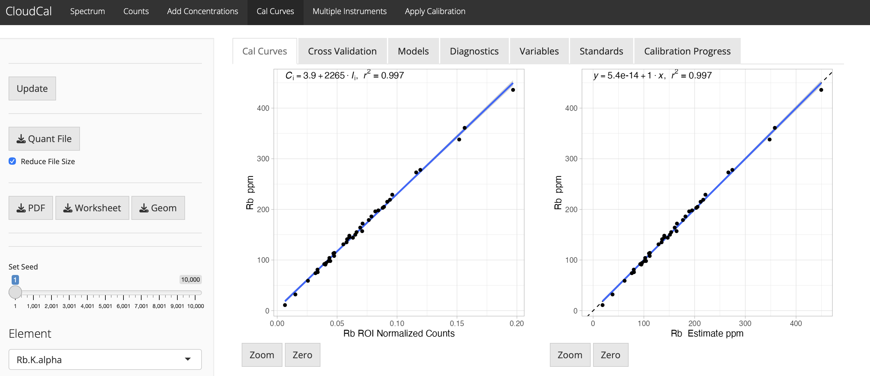
- Build Calibration: Select model type and train in Cal Curves tab
- Validate: Review cross-validation metrics and diagnostic plots
- Apply: Quantify unknowns in the Apply Calibration tab
- Go to Setup → Group Conversion
- Select directory with PDZ files
- Choose CSV as output format
- Enable Replace duration with live time (recommended)
- Process spectra normally
- Go to Export → All Results (not "All Results to Excel")
- This creates compatible CSV files
- PDZ v24: Classic Tracer format (IISD/IVSD/IIV+)
- PDZ v25: Tracer 5i format
- LiveTime normalization option available for dead time correction
- Upload
.spespectrum files - Optionally upload
.dflfile for accurate energy calibration - Without DFL, SPE header calibration values are used
Column structure: Energy, Spectrum1, Spectrum2, ... or melted format with Energy, CPS, Spectrum columns.
The .quant file is an open-source RDS format containing all calibration data. To inspect:
str(readRDS("your_calibration.quant"))$FileType # Source data format (CSV, PDZ, etc.)
$Units # Concentration units (%, ppm)
$LineDefaults # Line definitions for peaks
$Spectra # Full spectral data used for calibration
$Intensities # Extracted element intensities
$Values # Reference material concentrations
$Deconvoluted # Output from xrftools linear deconvolution
└─$Areas # Net peaks
└─$Spectra # Baseline-subtracted spectra
└─$Baseline # Baseline spectra (used for normalizations)
└─$Parameters # Arguments passed to deconvolution functions
$calList # Per-element calibration models
└─$Element
├─$Parameters
│ ├─$CalTable # Includes normalization instructions and model arguments
├─$Slope # Lucas-Tooth/ML slope variables
├─$Intercept # Lucas-Tooth/ML intercept variables
├─$StandardsUsed # Standards included in model
└─$Model # Trained model object
CloudCal is based on the Lucas-Tooth and Price (1961) algorithm with extensions for modern machine learning:
Ci = r0 + Ii[ri + Σ(rinIn)]
Where:
- Ci: Concentration of element i
- r0: Intercept (empirical constant)
- ri: Slope coefficient for element i intensity
- rin: Interelement correction coefficient (effect of element n on element i)
- Ii: Net intensity of element i
- In: Net intensity of interfering element n
This extends simple linear regression (y = mx + b) by accounting for matrix effects where one element's fluorescence influences another's measured intensity.
- Estimate concentrations from X-ray spectra
- Account for matrix variation in different sample types
- Enable cross-instrument comparability for reproducible results
Please cite CloudCal in publications:
Current Version:
Drake, B.L. 2025. CloudCal. GitHub. https://github.com/leedrake5/CloudCal. doi: 10.5281/zenodo.2596154
Legacy Version (v3.0):
Drake, B.L. 2018. CloudCal v3.0. GitHub. https://github.com/leedrake5/CloudCal. doi: 10.5281/zenodo.2596154
- Kuhn, M. 2008. Building predictive models in R using the caret package. Journal of Statistical Software 28(5): 1-26
- Liaw, A., Wiener, M. 2002. Classification and Regression by randomForest. R News 2(3): 18-22
- Lucas-Tooth, H.J., Price, B.J. 1961. A Mathematical Method for the Investigation of Interelement Effects in X-Ray Fluorescence Analysis. Metallurgia 64: 149-152
- Speakman, R.J., Shackley, M.S. 2013. Silo science and portable XRF in archaeology: a response to Frahm. Journal of Archaeological Science 40: 1435-1443
- Venables, W.N., Ripley, B.D. 2002. Modern Applied Statistics with S. Fourth Edition. Springer, New York. ISBN 0-387-95457-0
Issues and pull requests are welcome at https://github.com/leedrake5/CloudCal/issues
See LICENSE file for details.